
GAMERA-OP: A three-dimensional finite-volume MHD solver for orthogonal curvilinear geometries
Date:
The GAMERA-OP (Orthogonal-Plus) is a three-dimensional finite-volume magnetohydrodynamics solver on orthogonal curvilinear geometry. The solver advances magnetic fields with constrained transport, preserving $\nabla\cdot\mathbf{B}=0$ to machine precision, and uses geometry-consistent high-order reconstruction with an enhanced partial donor cell method limiter that accounts for geometry curvature. Flexible numerics include various numerical fluxes and time integrators. In cylindrical and spherical coordinates, angular momentum are preserved at round-off, and a ring-averaging treatment near the axis relaxes CFL constraints while maintaining divergence-free magnetic fields. Optional capabilities comprise the semi-relativistic (Boris) correction, background-field splitting, and anisotropic MHD formulation. Rewritten in C, the code adopts a modular design that simplifies case setup and facilitates adding physics and coupling to other first-principles codes. Standard benchmarks across multiple geometries verify accuracy, low numerical diffusion, and robust handling of coordinate singularities and rotating flows. GAMERA-OP provides a practical, high-order framework for space and astrophysical plasma applications where orthogonal curvilinear coordinates and exact angular-momentum conservation are advantageous.
Keywords: Numerical MHD, Finite Volume Method, Orthogonal Curvilinear Geometry
1 Introduction and History
Numerical simulations based on the magnetohydrodynamic (MHD) equations have long been a cornerstone for studying solar–terrestrial and astrophysical systems. Over recent decades, numerous well established MHD codes now support astrophysical and space physics studies, including ZEUS [1], Athena [2,3], PLUTO [4], NIRVANA [5], the Pencil code [6], FLASH [7], and BATS-R-US [8]. Adaptive mesh refinement (AMR) has increasingly been employed as an effective means to resolve phenomena with vastly different spatial and temporal scales [3,9], and high-order finite-volume methods have proven effective because they achieve higher accuracy at considerably lower cost relative to traditional second-order frameworks [10,11].
The Lyon–Fedder–Mobarry (LFM) MHD code, developed at the Naval Research Laboratory in the early 1980s, pioneered three-dimensional MHD in non-orthogonal curvilinear geometry with high-quality advection schemes. Its core design philosophy remains influential—employing a high-order reconstruction with constrained transport (CT) [12,13] to enforce $\nabla\cdot\mathbf{B}=0$ to machine precision. LFM has been coupled to additional physics components, e.g., including a magnetosphere–ionosphere (M–I) coupler [14] and the Rice Convection Model (RCM) for the inner magnetosphere [15], and applied to problems ranging from the inner heliosphere [16] to multifluid extensions [17,18]. The GAMERA (Grid-Agnostic MHD for Extended Research Applications) code [19] is a modern reinvention of LFM, retaining its strengths while significantly improving implementation, optimization, and numerical algorithms. GAMERA has been used extensively for the terrestrial magnetosphere [20], the inner heliosphere [21], giant-planet magnetospheres [22,23], and unmagnetized bodies via a multifluid extension [24].
In LFM and GAMERA, the governing equations are solved on non-orthogonal curvilinear meshes using a ingeniously designed Cartesian-based finite-volume formulation with coordinate transformations that cell-centered vector components are expressed in a global Cartesian basis regardless of the computational coordinate system. While elegant and effective, this design complicates extension to AMR and to higher-order finite-volume frameworks. In addition, the Cartesian-based update does not strictly conserve angular momentum, which is essential for rapidly rotating systems. By contrast, solving the equations intrinsically in orthogonal coordinates simplifies higher-order FV implementation, and orthogonal curvilinear systems—cylindrical, spherical, and modified dipole [25] admit exact angular momentum conservation.
Because ideal MHD simulation is a grid-scale fluid approximation, it cannot capture kinetic (particle-scale) physics; thus, coupling an MHD fluid solver to a subgrid/particle module is often desirable. However, the architecture of GAMERA makes such tight coupling, for example to particle solvers such as [26], comparatively inefficient. Motivated by these considerations, we introduce GAMERA-OP (Orthogonal-Plus), a successor to LFM/GAMERA rewritten from scratch in C (the predecessors were in Fortran). GAMERA-OP solves the MHD equations on arbitrary orthogonal curvilinear coordinates, adds extended physics modules, and incorporates improved numerical algorithms. It enforces solenoidal magnetic field condition via constrained transport on orthogonal geometry and conserves angular momentum to round-off using an angular momentum preserving discretization. A geometry-consistent, very high-order spatial reconstruction is employed. Extended MHD with anisotropic pressure is supported. GAMERA-OP further offers flexible time integration and flux options.
2 Numerical Schemes
2.1 Governing Equations
We solve the following set of single-fluid, normalized ideal MHD equations given by:
\[\frac{\partial \rho}{\partial t}=-\nabla \cdot(\rho \boldsymbol{u}) \tag{1}\] \[\frac{\partial \rho \boldsymbol{u}}{\partial t}=-\nabla \cdot(\rho \boldsymbol{u} \boldsymbol{u}+\overline{\boldsymbol{I}} P)+\boldsymbol{F_L} \tag{2}\] \[\frac{\partial \mathcal{E_P}}{\partial t}=-\nabla \cdot\left[\boldsymbol{u}\left(\mathcal{E_P}+P\right)\right]+\boldsymbol{u} \cdot \boldsymbol{F_L} \tag{3}\] \[\frac{\partial \mathcal{E_T}}{\partial t}= -\nabla \cdot\left[ \boldsymbol{u} \left(\mathcal{E_P} + P\right) +\boldsymbol{E} \times \boldsymbol{B}\right] \tag{4}\] \[\frac{\partial S}{\partial t}=-\nabla \cdot(S \boldsymbol{u}) \tag{5}\] \[\frac{\partial \boldsymbol{B}}{\partial t}=-\nabla \times \boldsymbol{E} \tag{6}\]where $\rho$, $\boldsymbol{u}$, $P$ are plasma density, bulk velocity and thermal pressure respectively. $\boldsymbol{F_L}=\nabla \cdot\left(\boldsymbol{B B}-\overline{\boldsymbol{I}} \frac{B^2}{2}\right)$ represents the Lorentz force and $\boldsymbol{B}$ is the magnetic field. $\boldsymbol{E}=-\boldsymbol{u} \times \boldsymbol{B}$ is the electric field from Ohm’s law. The quantities $\mathcal{E_P}$, $\mathcal{E_T}$ and $S$ denotes the plasma/hydrodynamic energy, total energy and entropy density defined as follows:
\[\mathcal{E_P} = \frac{1}{2} \rho u^{2}+\frac{P}{\gamma-1}\] \[\mathcal{E_T}=\mathcal{E_P} + \frac{B^2}{2}\] \[S= P \rho^{1-\gamma}\]where $\gamma$ is the ratio of the specific heat.
For most applications, as in LFM and GAMERA, the semi-conservative formulation based on the plasma energy equation ($\mathcal{E}_P$) is adopted as the default. This approach is especially robust in low-$\beta$ regimes, such as planetary magnetospheres and the solar corona, where the use of the total energy equation can easily lead to negative pressure due to strong magnetic dominance. The entropy equation is also included for improved stability and robustness in certain regimes.
2.2 Grid Definitions and Notations
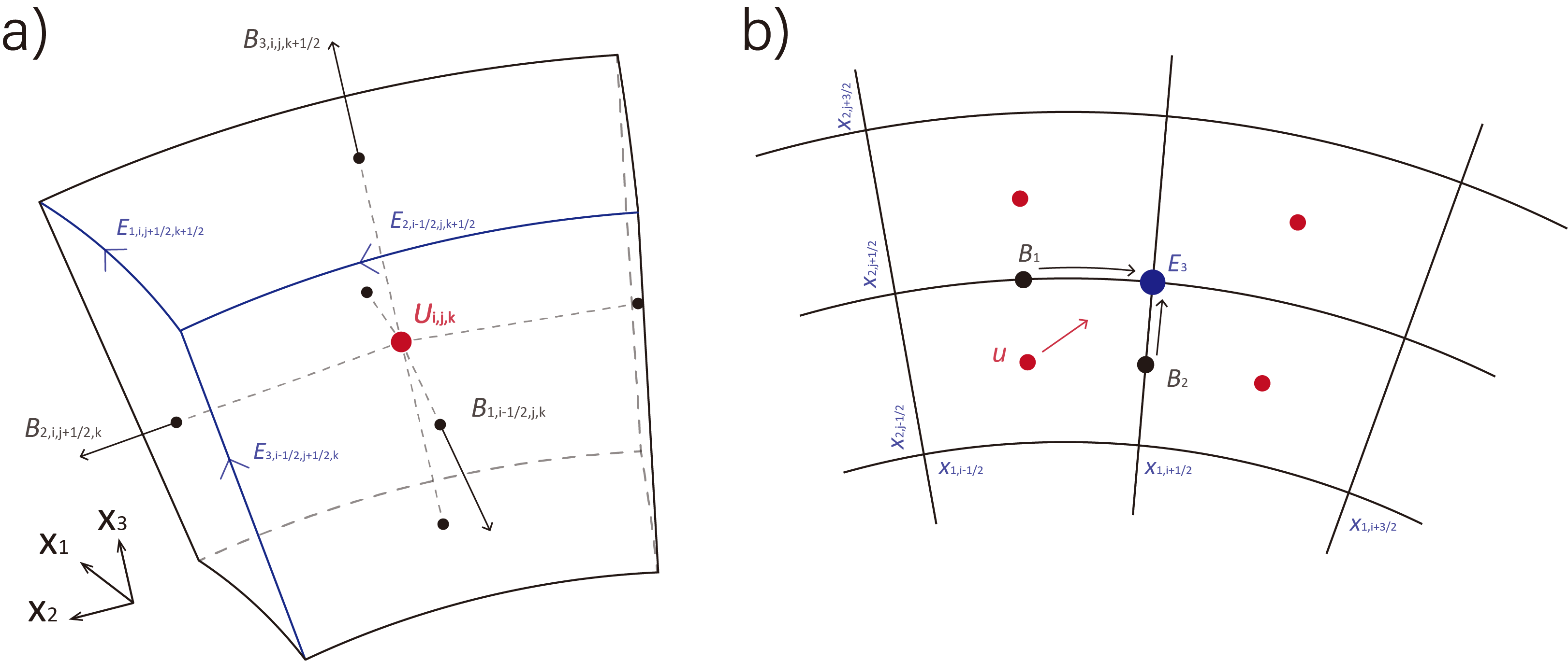
In this paper, we consider numerical schemes formulated in standard Cartesian, cylindrical, and spherical coordinate systems. The finite-volume computational cell labeled by indices $(i,j,k)$ is defined within the zone $[x_{1;i-\frac{1}{2}},x_{1;i+\frac{1}{2}} ] \times [ x_{2;j-\frac{1}{2}},x_{2;j+\frac{1}{2}} ] \times [ x_{3;k-\frac{1}{2}},x_{3;k+\frac{1}{2}}]$, where $(x_1, x_2, x_3)$ are the general computational space coordinates equal to $(x, y, z)$, $(R, \phi, z)$ and $(r, \theta, \phi)$ for Cartesian, cylindrical, and spherical coordinate, respectively. Edge lengths, face areas, and cell volumes are determined using appropriate geometric scale factors.
Table 1: The Grid Definitions and Index Notations Used in GAMERA-OP
| Grid Variable | Grid Location | Cartesian | Cylindrical | Spherical | Grid Index |
|---|---|---|---|---|---|
| $L_1$ | Cell Edges (1) | $\Delta x$ | $\Delta R$ | $\Delta r$ | $i , j + \frac{1}{2}, k + \frac{1}{2}$ |
| $L_2$ | Cell Edges (2) | $\Delta y$ | $R_{i+1 / 2}\Delta \phi$ | $r_{i+1 / 2}\Delta \theta$ | $i + \frac{1}{2}, j , k + \frac{1}{2}$ |
| $L_3$ | Cell Edges (3) | $\Delta z$ | $\Delta z$ | $r_{i+1 / 2}\sin \theta_{j+1 / 2} \Delta \phi$ | $i + \frac{1}{2}, j + \frac{1}{2}, k$ |
| $A_1$ | Cell Faces (1) | $\Delta y \Delta z$ | $R \Delta \phi \Delta z$ | $-r_{i+1 / 2}^2 \Delta \cos \theta \Delta \phi$ | $i+\frac{1}{2}, j, k$ |
| $A_2$ | Cell Faces (2) | $\Delta z \Delta x$ | $\Delta R \Delta z$ | $\frac{1}{2}\Delta r^2 \sin \theta_{j+1 / 2} \Delta \phi$ | $i, j+\frac{1}{2}, k$ |
| $A_3$ | Cell Faces (3) | $\Delta x \Delta y$ | $\frac{1}{2}\Delta R^2 \Delta \phi$ | $\frac{1}{2}\Delta r^2 \Delta \theta$ | $i, j, k+\frac{1}{2}$ |
| $V$ | Cell Volumes | $\Delta x \Delta y \Delta z$ | $\frac{1}{2}\Delta R^2 \Delta \phi \Delta z$ | $-\frac{1}{3} \Delta r^3 \Delta \cos \theta \Delta \phi$ | $i,j,k$ |
Note: Here the $\Delta$ symbol denotes the difference computed of the argument between its value at the upper and lower zone interfaces, e.g., $\Delta r^3 = (r_{i+1/2}^3 - r_{i-1/2}^3)$, and $\Delta \cos \theta = \cos \theta_{j+1/2} - \cos \theta_{j-1/2}$.
(a) The locations of the volume centered fluid variables $\boldsymbol{U}$, the face-centered magnetic fields $\boldsymbol{B}$, and the edge-centered electric fields $\boldsymbol{E}$. (b) A schematic showing the evaluation of the electric fields $E_3$ in a 2D slice ($x_1$-$x_2$ plane).